Modeling with cge_modeling#
A CGE model is comprised of three components:
Variables: symbolic objects that represent model quantities that will vary endogenously in your model.
Parameters: symbolic objects that represent model quantities that will vary exogenously in your model (or not at all!)
Equations: A mathematical description of your model economy.
To create a model, one first must write down all the variables and parameters that will go into the model.
Model Setup#
In this first simple model, we consider an economy with a single household and a single firm. The household has fixed endowments of labor and capital, which it sells to the firm for wages and rents, respectively. The firm uses these to produce a single consumption good, which it then sells back to the household. There is no government and no investment. The structure of the economy is shown in the following graph:
import graphviz as gr


def draw_graph(edge_list, node_props=None, edge_props=None, graph_direction="UD"):
    """Utility to draw a causal (directed) graph"""
    g = gr.Digraph(
        graph_attr={"rankdir": graph_direction, "ratio": "0.25"},
        engine="neato",
    )

    edge_props = {} if edge_props is None else edge_props
    for e in edge_list:
        props = edge_props[e] if e in edge_props else {}
        g.edge(e[0], e[1], **props)

    if node_props is not None:
        for name, props in node_props.items():
            g.node(name=name, **props)
    return g


nodes = ["K", "L", "Y", "C", "Household", "Firm"]
edges = [
    ("Household", "K_s"),
    ("Household", "L_s"),
    ("Household", "C"),
    ("Firm", "Y"),
    ("Firm", "K_d"),
    ("Firm", "L_d"),
    ("K_d", "Capital Market"),
    ("L_d", "Labor Market"),
    ("K_s", "Capital Market"),
    ("L_s", "Labor Market"),
    ("C", "Goods Market"),
    ("Y", "Goods Market"),
]
edge_props = {
    ("K_d", "Capital Market"): {"label": "r"},
    ("K_s", "Capital Market"): {"label": "r"},
    ("L_d", "Labor Market"): {"label": "w"},
    ("L_s", "Labor Market"): {"label": "w"},
    ("C", "Goods Market"): {"label": "P"},
    ("Y", "Goods Market"): {"label": "P"},
}
draw_graph(edges, edge_props=edge_props, graph_direction="LR")

Given this structure, the economy will be comprised of the following equations:
Since we are an endowment economy, we take \(K_s\) and \(L_s\) as given – they are thus parameters. The variables are \(Y\), \(C\), \(K_d\), \(L_d\), \(w\), \(r\), and \(P\). \(\Pi\), the profits of the firm, we set to zero to eliminate. So we have 7 variables and 7 unknowns.
Underdetermination#
The system above looks square, but actually it’s not! The household budget constraint is equivalent to the goods market clearning condition. To see this, you have to know that the equations for the firm’s factor demand are based on the zero profit condtion. Suppose we don’t eliminate \(\Pi\), and instead use the identity:
Substituting this into the household budget constraint, we obtain:
From the factor clearing conditions we have \(K_d = K_s\) and \(L_d = L_s\), so we can make these substitutions:
We recovered the market clearing condition from the other equations! This shows that although we wrote down 7 equations, we actually only have 6 equations worth of information.
Walras’ Law and Choice of Numeraire#
It’s surprising that we only have 6 independent equations, given that we have 7 variables. But actually we only have 6 variables. This is because of Walras’ law. The law says that, given perfect competiton and flexible prices in all markets (which we’ve assumed), the sum of the values of excess demands (or supplies) must be zero. This is an additional constraint on the economy, which has the effect of pinning down the price of the last good, assuming we know the prices of all other goods. In our case, if we know values of \(r\) and \(w\), we are not free to choose a value for \(P\).
As a result, one of our prices is not actually a variable at all. We are required to choose a numeraire – a price that all other prices are measured by. The choice of numeraire is the modeler’s. I will choose \(w\), the wage level, to be the numeraire. As a result, all prices will be expressed in hourly wages.
Conceptually, we think of \(w\) as a parameter now (which we will fix to be 1 – since any numeraire value implies a valid price vector, we might as well choose the easiest possible value). Now we have 6 variables are 7 equations, 6 of which are independent.
Squaring up the system#
Now we just need to make the system square. We have two choices. First, we could remove one of the redundant equations (either the household budget constraint or the goods market clearing conditions). Alternatively, we can add a dummy “residual” variable, which we set to zero. This second choice is popular because it adds a consistency check to model simulations. This residual should always be zero, at all valid equlibria.
We will add a residual term, \(\varepsilon\), to the market clearing condition. So our system now becomes:
The Final System#
Finally, we need to specify a production function. We can use Cobb-Douglas, so \(Y = f(K_d, L_d) = AK_d^\alpha L_d^{1-\alpha}\).
The system then becomes:
Where \(Y\), \(C\), \(K_d\), \(L_d\), \(r\), \(P\), and \(\varepsilon\) are variables. \(A\), \(\alpha\), \(L_s\), \(K_s\), and \(w\) are parameters.
We have 7 variables and 7 independent equations (since the market clearing and budget constraint now vary by \(\varepsilon\)!), and we are ready to proceed.
Declare Variables#
First, we make a list of variables using the Variable class. In their simplest form, variables have a name and a description. We can optionally also specify a latex_name for pretty printing.
variables = [
    Variable("Y", description="Total output"),
    Variable("C", description="Household constumption"),
    Variable("K_d", description="Firm demand for capital"),
    Variable("L_d", description="Firm demand for labor"),
    Variable("r", description="Rental rate of capital"),
    Variable("P", description="Price of consumption goods"),
    Variable("resid", latex_name="\\varepsilon", description="Walrasian residual"),
]
Declare Parameters#
Parameters are exactly the same as Variables, except that they are treated differently inside the model.
parameters = [
    Parameter("A", description="Total factor productivity"),
    Parameter("alpha", description="Share of capital in production"),
    Parameter("L_s", description="Household endowment of labor"),
    Parameter("K_s", description="Household endowment of capital"),
    Parameter("w", description="Wage level"),
]
Declare equations#
Equations also have a name, but instead of a description, you need to provide a string form of the equation.
equations = [
    Equation("Production function", "Y = A * K_d ** alpha * L_d ** (1 - alpha)"),
    Equation("Firm capital demand function", "K_d = alpha * Y * P / r"),
    Equation("Firm labor demand function", "L_d = (1 - alpha) * Y * P / w"),
    Equation("Household budget constraint", "P * C = r * K_s + w * L_s"),
    Equation("Labor market clearing", "L_s = L_d"),
    Equation("Capital market clearing", "K_s = K_d"),
    Equation("Goods market clearing", "Y = C + resid"),
]
Create a model#
With these these lists, we are ready to create a CGEModel
mod = cge_model(variables=variables, parameters=parameters, equations=equations)
Initial pre-processing complete, found 7 equations, 7 variables, 5 parameters
Once the model is built, we can look at the equations
mod.equation_table()
As well as the parameters and variables
mod.summary("variables")
mod.summary("parameters")
Or, if you prefer, everything together
mod.summary()
Data and Calibration#
To actually run policy experiments, you have to first find a non-trivial model equlibrium. To check for an equlibrium, you can use the model.check_for_equlibrium method. It expects a dictionary containing all model variables and parameters, and checks whether all provided model equations are equal to zero
Equilibrium not found. Total squared error: 34.004656


Equation                              Residual
====================================================================================================
Production function                   -0.084686
Firm capital demand function           1.923461
Firm labor demand function             0.022343
Household budget constraint           -3.172644
Labor market clearing                  4.451211
Capital market clearing               -0.481453
Goods market clearing                 -0.431901
For data, we will use a (fake!) balanced SAM. We exploit the fact that the SAM is balanced to “calibrate” the model, choosing parameter values that lead to the data observed in the SAM. Calibration is unique to each model, so cge_modeling currently can’t do that for you. What it can do is help you with some consistency checks. We need to:
Write a python function that takes the model, plus all required initial data from the SAM
Inside the function, make sure every parameter and variable is given a value
return
model.check_calibration()
model.check_calibration() specifically looks at the local namespace, so it’s important that it is called from within a function.
Load Data#
import pandas as pd

sam = pd.read_csv("../data/simple_rbc_data.csv", index_col=[0, 1], header=[0, 1]).fillna(0)
sam
| Factor | Institution | Production | Activities | |||
|---|---|---|---|---|---|---|
| Labor | Capital | Household | Firm | Firm | ||
| Factor | Labor | 0.0 | 0.0 | 0.0 | 0.0 | 7000.0 |
| Capital | 0.0 | 0.0 | 0.0 | 0.0 | 3000.0 | |
| Institution | Household | 7000.0 | 3000.0 | 0.0 | 0.0 | 0.0 |
| Production | Firm | 0.0 | 0.0 | 10000.0 | 0.0 | 0.0 |
| Activities | Firm | 0.0 | 0.0 | 0.0 | 10000.0 | 0.0 |
First we can double check that this is a properly balanced SAM by checking that the sum of the rows is equal to the sum of the columns
sam.sum(axis=1) == sam.sum(axis=0)
Factor       Labor        True
             Capital      True
Institution  Household    True
Production   Firm         True
Activities   Firm         True
dtype: bool
For bigger SAMs its not realistic to look row by row, so we can use .all()
(sam.sum(axis=1) == sam.sum(axis=0)).all()
True
Next, we extract the required initial values. In this case we actually know basically everything, but let’s try to work with the minimum set: \(Y\), \(K_d\), \(L_d\).
initial_values = {
    "Y": sam.loc[("Activities", "Firm"), ("Production", "Firm")],
    "K_d": sam.loc[("Factor", "Capital"), ("Activities", "Firm")],
    "L_d": sam.loc[("Factor", "Labor"), ("Activities", "Firm")],
}
initial_values
{'Y': 10000.0, 'K_d': 3000.0, 'L_d': 7000.0}
Calibration#
Now that we have data, we need to “calibrate” the CGE model to the data. Calibration is process in which we use observed values in the same to calculate parameter values. All widely used production and utility functions have off-the-sheft calibration equations for all or most of the parameters. In the case of the Cobb-Douglas production function, the calibrating equations are:
It is easy to see that the second equation is just a re-arrangement of the production function, conditional on knowing the value of \(\alpha\). The equation for \(\alpha\) itself comes from “inverting” the factor demand functions:
A sidenote on prices#
To perform this calibration, we need to know \(K_d\), \(L_d\) , and \(Y\). It is tempting to read these values off from the SAM. After all, it records transfers from the activity account (the firms’ purchases of inputs) to the factor accounts (e.g. \(K_d\) and \(L_d\)) as well as flows from the production account to the activity account (the firm’s output). Recall though that the SAM records the value of these flows – that is, \(\text{Price} \times \text{Quantity}\).
When computing \(\alpha\) the situation isn’t so bad, because all terms enter as values. That is, we have \(rK_d\) and \(wL_d\), and never \(K_d\) or \(L_d\) (the quantity variables) alone. But for computing \(A\), we do need to pick apart the price and quantity. Since we’re unlikely to have access to detailed price data, trickery will be employed.
The trick in this case is called “normalization”. To understand the trick, first realize that “quantity” is a value with units. We might not know what these units are without digging into statistical documentation, but the SAM might record, for example, purchases of wheat by households from wheat farmers in bushels. So the value \(V = PQ\) in this case would be \(\text{Currency} \times \text{Bushel}\).
Note that this choice of unit is entirely arbitrary. If we knew the price of a kilogram of wheat instead, we could just as easily have reported \(V = P^\prime Q^\prime\), with \(P^\prime Q^\prime\) measured in \(\text{Currency} \times \text{Kilograms}\). Importantly, though, the total value would be the same – note that I did not write \(V^\prime\) in the 2nd equation; this was delibrate!
Given this, there is a sense in which we are free to choose whatever units we wish, as long as we are consistent. Let us choose the most convenient unit possible – the “Unit Currency Unit”. That is, we choose whatever unit of every good, such that the price of that good is exactly 1 unit of currency. Labor is measured in whatever fraction of time such that the wage for that time is one dollar. Cars are measured in fractional cars, such that the price of the fraction is one dollar, and so on.
This might strike you as a bit silly, but you have to admit it’s very convenient! We are now free to set \(P=1\), and \(r=1\) (recall that we already set \(w=1\), since it was chosen to be the numeraire). What changes is our interprertation. We cannot report “natural” units on the outputs of our simulations, since everything will be measured in “Unit Currency Units”. But not all hope is lost, because percentages are unitless! So we can calibrate to this odd unit, then report the results of a policy experiment in percentages.
Implementing the calibration#
Now we know how to actually do the calibration. We will:
Read in the necessary values from the SAM, in this case \(Y\), \(K_d\), and \(L_d\).
Normalize all prices to 1.
Calibrate \(\alpha\) and \(A\) using the formulas derived above
Compute all variables using model equations
cge_modeling provides a few tools to help you accomplish this. First, when setting constant values, you can use model.initialize_parameter. This will take care of shapes automatically for models with many dimensions. Second, you can use model.finalize_calibration. This will automatically collect the variables in a function context, check shapes, and return a dictionary of results. If anything was not declared, it will give a reminder.
The following cell shows how to use this features to calibrate our model. resid has been purposely omitted, to show how finalize_calibration will alert us to missing variables or parameters
def calibrate_model(mod, *, Y, K_d, L_d):
    # Normalize prices
    r = mod.initialize_parameter("r", 1.0)
    w = mod.initialize_parameter("w", 1.0)
    P = mod.initialize_parameter("P", 1.0)

    # Calibrate parameters
    alpha = r * K_d / (r * K_d + w * L_d)
    A = Y / K_d**alpha / L_d ** (1 - alpha)

    # Market clearing conditions
    K_s = K_d
    L_s = L_d
    C = Y

    return mod.finalize_calibration()
calibrated_values = calibrate_model(mod, **initial_values)
resid not found in model variables
Oops, we forgot resid. Let’s go back and fix it:
def calibrate_model(mod, *, Y, K_d, L_d):
    # Normalize prices
    r = mod.initialize_parameter("r", 1.0)
    w = mod.initialize_parameter("w", 1.0)
    P = mod.initialize_parameter("P", 1.0)

    # Calibrate parameters
    alpha = r * K_d / (r * K_d + w * L_d)
    A = Y / K_d**alpha / L_d ** (1 - alpha)

    # Market clearing conditions
    K_s = K_d
    L_s = L_d
    C = Y
    resid = Y - C

    return mod.finalize_calibration()
In Python, no news is good news!
calibrated_values = calibrate_model(mod, **initial_values)
We can check that the calibrated values have zero residual when plugged into the model equations
mod.check_for_equilibrium(calibrated_values)
Equilibrium found! Total squared error: 0.000000
We have an equlibrium. We can now proceed to policy simulation
Policy Simulation#
To perform a policy simulation, use the simulate method. This method has a number of options, but the most important are the following:
initial_stateis the initial equilibrium from which to begin. In most cases this will be the calibrated equlibrium, but it could also be a previous simulation (if you’re doing recursive modeling through time, for example)final_delta,final_delta_pct, orfinal_valuesare how you specify the policy simulation. Ultimately, what you need to provide is a vector of final parameter values – the policy to be simulated. Each of these options are available to help you better reason about that. Values passed tofinal_deltaare added to the inital parameter values; values passed tofinal_delt_pctare multiplied by the initial values; andfinal_valuescompletely override the initial values.Suppose the initial value of labor supply was 1000, and we want to simulate a cut in labor supply to 500. The following specifications are all equivalent:
final_values={'L_s':500}final_delta={'L_s':-500}final_delta_pct = {'L_s':0.5}
use_euler_approximationanduse_optimizer. By default,cge_modelingsolves for the policy solution in two ways:Linearize the model, and convert the policy shock into an implicit ODE. This is “euler approximation”. Given infinite compute, it always gives the right answer, but involves some expensive matrix inversion. As a bonus, it gives you all equlibria on the way from the initial state to the final state, so you can see a small slice of the function space.
Solve for the new equlibrium using a numerical routine. This can be more direct, but sometimes struggles on complex problems.
The strategy of
cge_modelingis to use the euler approximation with a conservative number of steps to move the model into the neighborhood of the solution, then use a numerical optimizer to finish the job. You acn disable one or the other, though, if you don’t want to use both.optimizer_mode, one ofrootorminimize.rootsolves for a vector of zeros directly, using multivariate root finding algorithms.minimizetries to minimize the sum of squared residuals using some flavor of Newton’s Method. Usuallyrootworks fine, but on really stubbon problemsminimizeis nice to try.
Other options are related to saving and loading model results. Any other keyword arguments are passed to the scipy optimizer being used, so check the scipy documentation to learn what you can do there.
50% Labor Supply Reduction#
We now (finally) run a policy simulation, to study what happens if households work 50% less. I use the final_delta_pct argument to directly specify the cut in percentage terms.
labor_cut = mod.simulate(
    initial_state=calibrated_values,
    final_delta_pct={"L_s": 0.5},
    optimizer_mode="minimize",
    use_euler_approximation=True,
)
We get back a dictionary with three entries. euler and optimizer hold xarray objects with the results of their respective optimization steps. optim_res holds the raw optimizer result returned by scipy. We can see from the optim_res that optimization was successful. We can also see that during Euler approximation, the errors in the approximation stayed around 0.01, which is good.
labor_cut["optim_res"]
 message: Optimization terminated successfully.
 success: True
  status: 0
     fun: 1.2798018880756698e-17
       x: [ 6.156e+03  6.156e+03  3.000e+03  3.500e+03  5.000e-01
            8.123e-01  9.196e-09]
     nit: 6
     jac: [-4.780e-09  1.915e-09  1.009e-09  3.417e-09  2.728e-09
           -1.680e-09  3.165e-09]
    nfev: 7
    njev: 7
    nhev: 33
It’s also good to check the final value of the resid variable, since we know it should always be zero. If it isn’t, we have a problem in our model closure.
labor_cut["optimizer"].variables["resid"]
<xarray.DataArray 'resid' (step: 2)> Size: 16B
array([0.00000000e+00, 9.19615331e-09])
Coordinates:
  * step     (step) int64 16B 0 1
Plotting#
cge_model.plotting offers some plotting functions to examine outputs. The two most important are plot_bar and plot_line. See the example gallery for how to use these.
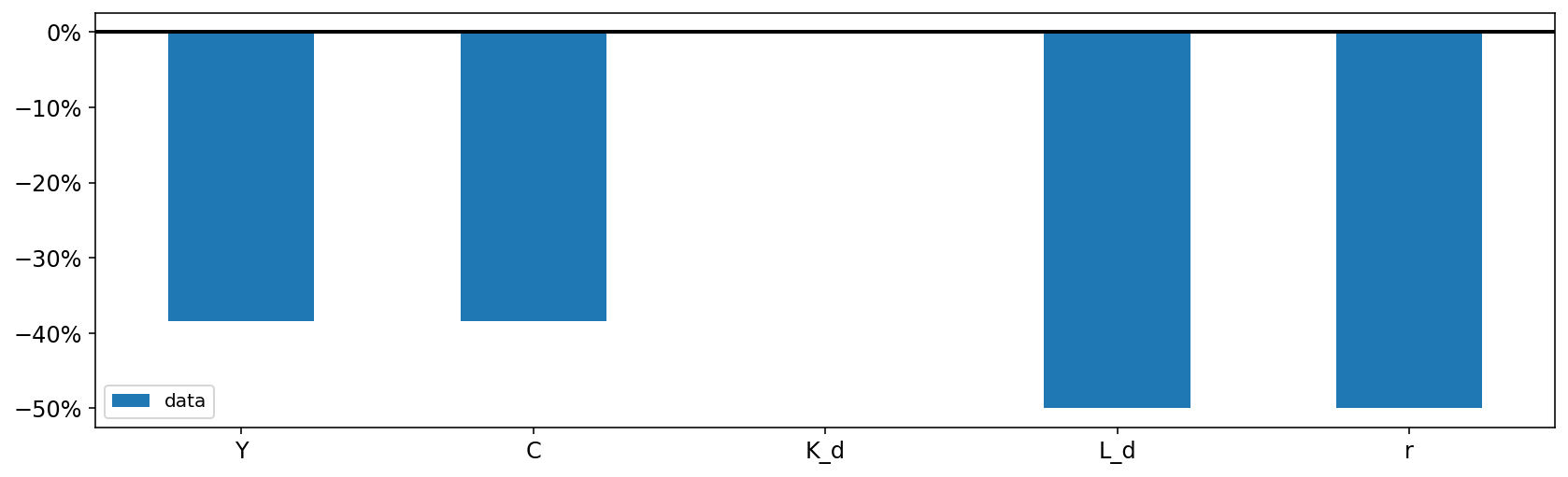
First, we can look at the total change from the initial to the final state using gcp.plot_bar. Since all of the variables have the same dimensions (in this case, no dimensions!) we set plot_together = True to see all the plots on a single axis.
The default is to plot each variable in its own axis, which makes sense when the variables have different dimensions (for example, one is defined over the set of firms, and other over the set of households).
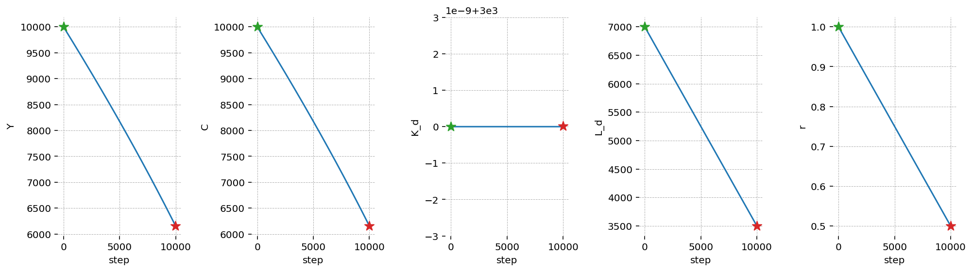
In this case, real demand for capital \(K_d\) did not change. This is because it was the price of capital \(r\) that shifted in response to the reduced labor supply. Capital becomes relatively cheaper as wages go up (remember that implicity \(r = \frac{r^N}{w}\), since wages are the numeraire!), and the net effect is no change to capital demand.
On the other hand, the budget line for the household shifts inward (because their endowment of labor has been reduced), which decreases consumpton (and output, which is the same thing in this economy).
cgp.plot_bar(
    labor_cut,
    mod,
    var_names=["Y", "C", "K_d", "L_d", "r"],
    plot_together=True,
    figsize=(14, 4),
    legend=True,
    metric="pct_change",
);
Thanks for the Euler Approximation approach, we can also trace out the effect of each “step” in the labor supply reduction on all the other variables. We can see this with plot_lines.
In this case, we see that the reduction in all variables is essentially linear in the labor supply. This makes sense, since the driving effect is the shifting inward of the household budget constraint.
cgp.plot_lines(labor_cut, mod, var_names=["Y", "C", "K_d", "L_d", "r"], figsize=(14, 4));